
The genome of all somatic cells (except B-lymphocytes) in an organism is the same; however, cells have varied functions and differ from one another. How do these differences take place? Why do only red blood cells (RBCs) make hemoglobin, and why do only certain pancreatic cells create insulin? The answer lies in their genome expression, known as differential gene expression.
What is Differential Gene Expression Analysis?
Differential gene expression (DGE) analysis can be defined as the process of identifying and analyzing differences in gene expression levels between two or more biological conditions. Gene expression is quantitative (i.e., low or high levels of expression) depending on the cellular response to signals or triggers. To elaborate, once an embryonic stem cell divides into more specialized cells, the potency of differentiation is lost. The genes of stem cells are switched off, and those required for the specialized function are switched on. The cells express different phenotypes but with the same genotype on the basis of their external environmental conditions.
In the past, gene expression was studied by using low-throughput methods, such as quantitative PCR (qPCR), northern blotting, which are limited to a single transcript of RNA. The microarray was developed for high-throughput quantification of gene expression, but it was restricted to known genes, relatively time-consuming, and expensive. Presently, RNA-sequencing methods are used to analyze the transcriptome of the cells. It is now the gold standard for modern DGE analysis.
Steps of Differential Gene Expression Analysis for RNA Sequencing
The entire workflow of differential gene expression involves sample collection, RNA extraction and sequencing, quality control, quantification, normalization, statistical testing, visualization, and functional analysis. It is to be noted that DGE can be purely computational; the RNA sequencing data are available in databases such as NCBI, GEO, etc.
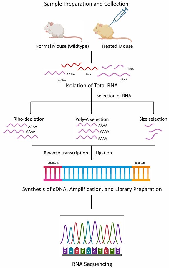
Sample collection
- The sample collection usually involves cells or tissues of organisms. Since there are over 200 different cell types with more than 50 organs in humans alone, the choice of sample should not be random and should be research-driven.
- DGE analysis experiments are designed in such a way as to compare control and experimentally-altered groups. Both groups must have similar times of collection, tissue/cell specificity, developmental stage, matched age, sex, batch, and environmental conditions to avoid error and bias.
- DGE experiments usually comprise at least two or three biological replicates for each group.
RNA Extraction
- The total RNA content of the cell is isolated and extracted from the biological samples using high-quality RNA extraction methods such as magnetic bead-based methods, column-based methods, or even phenol-chloroform methods (with the use of TRIzol). Each of these steps has its benefits and cons.
- The concentration and quality of isolated RNA can then be determined by using a Nanopore/spectrophotometer.
- As RNA is unstable, it must be stored at -80 °C or flash-frozen to -196 °C immediately after isolation.
Selection of RNA Species
- The total RNA contains ribosomal RNA (rRNA), precursor messenger RNA (pre-mRNA), mRNA, and other non-coding RNA (ncRNA).
- Depending on the objective of the experiment, RNA species can be selected by using poly-T oligos, magnetic beads, rRNA depletion, miRNA enrichment, and RNA capture.
- The selection of poly-A RNAs is the most common, as most experiments are designed for comparing coding mRNA transcripts.
cDNA Synthesis and Library Preparation
- The isolated RNA is converted to cyclic DNA (cDNA) for more stability using the reverse transcriptase enzyme.
- They are amplified by using the polymerase chain reaction (PCR).
- The amplified cDNA is fragmented into smaller pieces and is ligated with adapters or tagged with deoxy-UTP (dUTP) for RNA sequencing.
RNA Sequencing
- Most researchers use single-end RNA sequencing to study gene expression, meaning the RNA transcripts are only read from one side.
- High-throughput RNA sequence methods involve mRNA sequencing for all protein-coding transcriptome, targeted RNA sequencing for specific genes, single-cell RNA sequencing for studying heterogeneous populations of cells, total RNA sequencing for coding and non-coding RNA, and small RNA sequencing for microRNAs.
- The sequencing generates raw data in the form of FASTQ format.
Quality Control and Preprocessing of Raw Reads
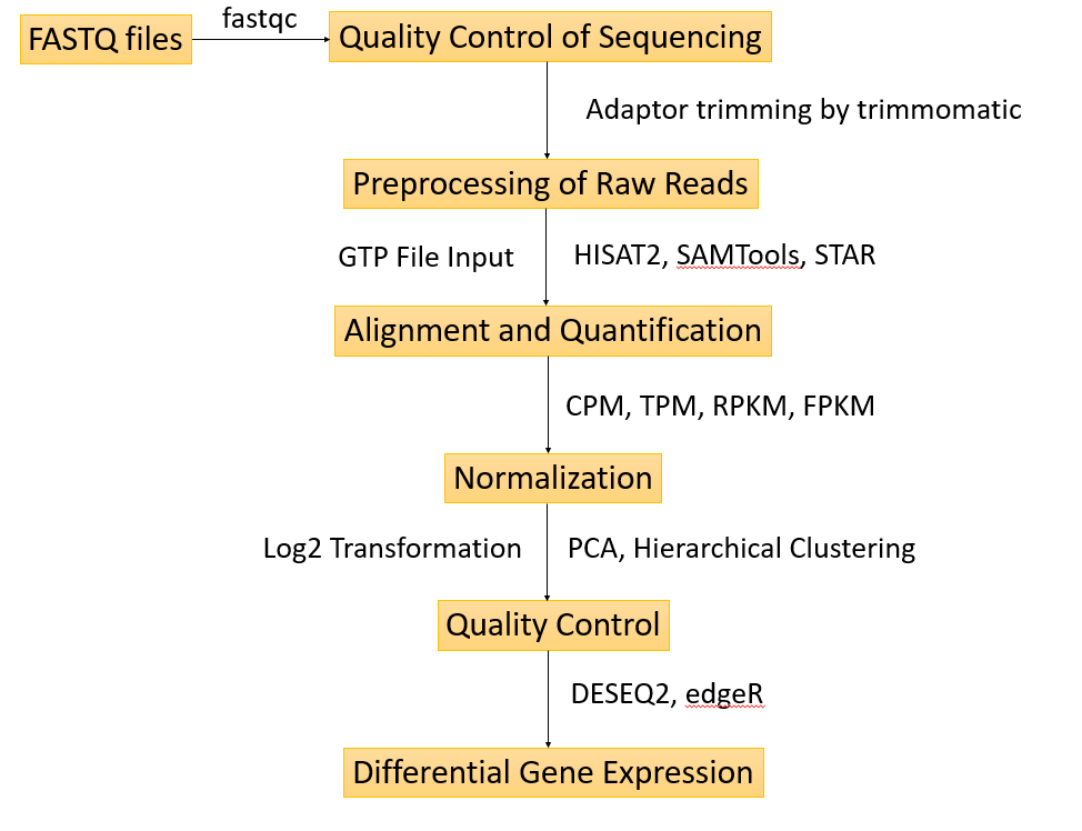
- The raw sequenced data needs to be assessed for quality to determine low-quality reads, adaptor contamination, microbial contamination, read length, etc., by using FASTQC and MULTIQC.
- The adaptors are removed using pipelines such as trimmomatic, fastp, or others.
Alignment and Quantification
- The quality-checked FASTQ files are then aligned and mapped with the reference genome using HISAT2, TopHAT, STAR, SAMtools, etc. The generated data is in the format of BAM files.
- A few times, the sequences do not align with the reference exons; such sequences are checked for quality control by RSeQC.
- Finally, the aligned sequence is quantified by using HTSeq. This results in a read count table in TSV file format with the genes and their counts.
- The count file is made into a table by the Define NGS Experiment.
Normalization
- The transcript counts must be normalized by gene length, sequencing depth, and total number of mapped reads to minimize error caused by the counting of genes.
- This is done by CPM (counts per million) for sequencing depth, TPM (transcripts per kilobase million) for depth and gene length, RPKM (Reads Per Kilobase of transcript per Million mapped reads) for single-end reads, and FPKM (Fragments Per Kilobase of transcript per Million mapped reads) for paired-end reads. However, the method can differ for the type of experiment, whether it’s a comparison or others.
- The counts are averaged for each of the technical replicates, whereas they are quantile-normalized for each set of biological replicates.
Quality Control
- After normalization, the next step includes sample-level and gene-level quality control. At this stage, the main objective is to examine the similarities and differences between the normalized data. It is to validate which of the samples (genes) have shown differential expression.
- Here, the log2 transformation to assess similarity, differences, and statistical significance of gene expression between samples using Principal Component Analysis (PCA) and hierarchical clustering.
Differential Gene Expression
- The final step is to fit the gene expression data from all qualified genes into a distribution model. Since the number of genes is very large (tens of thousands), expression values are not normally distributed. Therefore, generalized linear modeling and the negative binomial distribution are used. Additionally, gene expression values vary from gene to gene, making it nearly impossible to interpret when additional variables such as gender, batch, treatment, etc., are considered.
- For this, R programming packages in Bioconductor, such as DESeq2 and edgeR, are popular. These statistical packages use negative binomial distributions to analyze the data.
The following are the software/pipelines commonly used for differential gene expression (DGE):
| Process | Software/Pipeline | File |
| Sequencing Quality Control | FASTQC, MULTIQC | FASTQ |
| Removal of Adaptor | Fastq, trimmomatic | FASTQ |
| Alignment and Mapping | HISAT2, TopHAT, STAR, SAMtools | BAM |
| Quantification | HTSeq | Read count file (TSV) |
| Combine all the Count files into a Table | Define NGS Experiment | Read count table (TSV) |
| Normalization | CPM, TPM, RPKM/FPKM, | |
| Quality Control (PCA, clustering) | DESeq2 | |
| Differential Expression Analysis | DESeq2, edgeR | Gene lists (TSV) |
Graphical Interpretations of Differential Gene Expression for RNA Sequencing
Principal Component Analysis (PCA)
- Principal component analysis (PCA) is a dimensionality reduction technique used to identify the most significant variations and patterns in a dataset.
- It simplifies complex data sets by preserving the most important structures. PCA transforms a data set into a set of orthogonal components, known as principal components. The principal components with the highest variance are PC1, followed by PC2, and so on.
- Similar datapoints (co-related genes) cluster together, and those with no correlation lie apart.
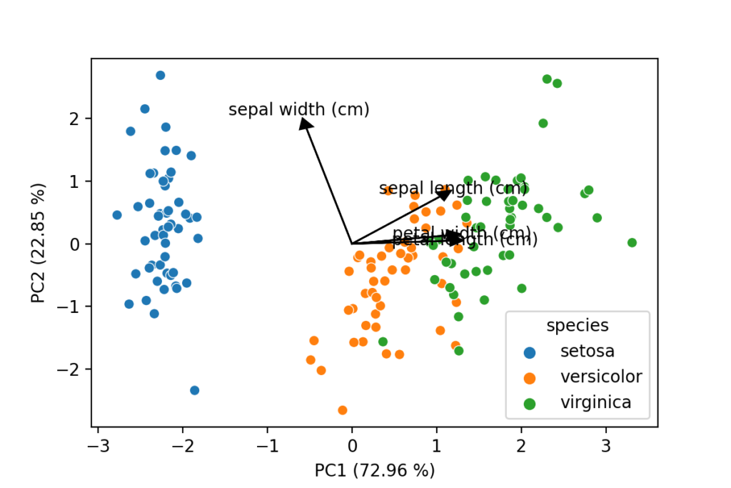
Figure 3 represents PCA of the famous iris dataset containing three species of iris flowers (setosa, versicolor, and virginica). The x-axis (PC1) has 72.96% variance, whereas the y-axis (PC2) has 22.85% variance (a total of 95% variance). Each colorful point is a flower sample, with setosa having the most distinct cluster. This means that setosa has the most distinguishable measurements compared to the iris flowers. The vector lines represent the direction and magnitude of the PC. To elaborate, sepal width is mostly upward, meaning that it contributes more to PC2, whereas the rest contribute more to PC1. Similarly, as the angle between petal length and petal width is small, meaning they have a strong correlation.
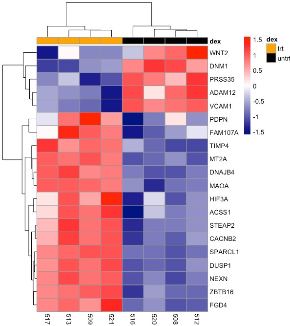
Hierarchical Clustering Heatmap
- Hierarchical clustering heatmap is a graphical representation for identifying strong patterns in a dataset with colors. In RNA sequencing, heat maps are coupled with dendrograms (used in phylogeny) to draw similarities or differences between the values.
- Hierarchical clustering heatmap displays the correlation of gene expression for all pairwise combinations of samples in the dataset.
- Samples generally have a high correlation with each other (values greater than 0.80) because the majority of the genes are not differentially expressed. Values lower than 0.80 could be outliers in the data or sample contamination.
In Figure 4, the horizontal rows represent the name of the sample; the vertical rows represent the name of the genes; the dendrogram horizontally and vertically represents the clustering of samples and genes, respectively; the color gradient indicates the level of expression of genes. Lastly, the blue and black tiles represent the two sample types for comparison.
Volcano Plot
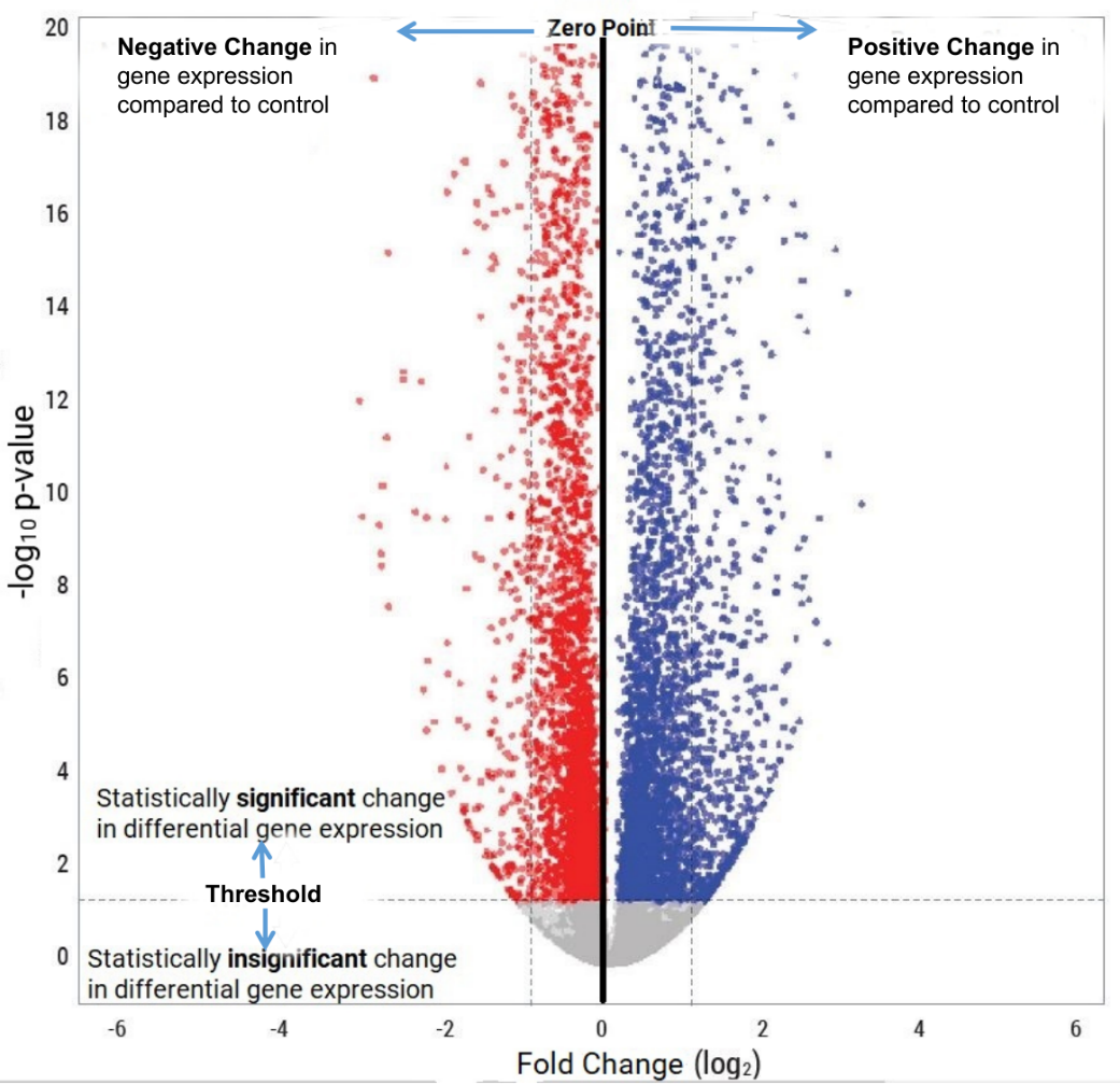
- A volcano plot is a graphical representation used to visualize the statistical significance of high-dimensional biological data, like gene expression.
- It indicates genes that are significantly differentially expressed between two experimental conditions. This is achieved simultaneously by displaying both the statistical significance (p-value) and the biological relevance (fold change) of each data point.
Key Components of Volcano Plot:
- Fold Change (FC): The x-axis of the plot represents fold change in gene expression between two conditions. It quantifies the increasing or decreasing level of gene expression. The point at the farthest (left or right) end signifies a substantial increase or decrease in gene expression.
- Statistical Significance (p-value): The y-axis represents the statistical significance of the differential expression. It is normally measured by statistical tests like the t-test or ANOVA. Data points with a threshold (mostly 0.05) are considered to be statistically significant.
With this, the volcano plot can be divided into four regions as follows:
- Upper Right Quadrant: The datapoints (genes) in this region are the most interesting candidates because they have a significant fold increase and are statistically significant.
- Upper Left Quadrant: The genes in this region have a significant fold decrease but are not statistically relevant.
- Lower Right Quadrant: The genes in this region are statistically significant but do not show a greater fold change. These genes could have limited biological importance, but still could be relevant if they are part of a larger regulatory network.
- Lower Left Quadrant: This region comprises genes that are neither biologically nor statistically relevant.
Applications of Differential Gene Expression Analysis for RNA Sequencing
Disease Discovery
Gene expression is crucial in understanding the molecular structure of diseases. DGE analysis is commonly used to determine how gene activity changes in response to various conditions, like the introduction of novel drugs in model organisms. These studies can lead to the identification of novel diagnostic markers and therapeutic targets.
Environmental Studies
DGE analysis can be used to study the response of organisms against environmental stressors like toxic substances, heavy metals, extreme temperatures, pollutants, carcinogens, or pathogens to better understand the response mechanism behind such impacts. By comparing the expression patterns of exposed and unexposed organisms, we can identify stress-response pathways/genes involved in immune defense, oxidative stress, DNA repair, etc. This helps to monitor the ecosystem by providing molecular indicators and might have potential roles in how genes might have evolved in an environment.
Development and Differentiation
Differential gene expression is widely used to study genes involved in embryonic development and cell differentiation. It plays a crucial role in determining the specific functions of each cell type. Because of this reason, gene expression-related studies in stem cell differentiation, regeneration, embryogenesis, etc., are popular.
References
- A comparison of mRNA sequencing (RNA-Seq) library preparation methods for transcriptome analysis | BMC Genomics | Full Text. (n.d.). Retrieved July 1, 2025, from https://bmcgenomics.biomedcentral.com/articles/10.1186/s12864-022-08543-3
- Differential gene expression (DGE) analysis. (n.d.). Training-Modules. Retrieved July 1, 2025, from https://hbctraining.github.io/Training-modules/planning_successful_rnaseq/lessons/sample_level_QC.html
- EMBL-EBI. (n.d.). Differential gene expression analysis | Functional genomics II. Retrieved July 1, 2025, from https://www.ebi.ac.uk/training/online/courses/functional-genomics-ii-common-technologies-and-data-analysis-methods/rna-sequencing/performing-a-rna-seq-experiment/data-analysis/differential-gene-expression-analysis/
- Gilbert, S. F. (2000). Differential Gene Expression. In Developmental Biology. 6th edition. Sinauer Associates. https://www.ncbi.nlm.nih.gov/books/NBK10061/
- How to employ statistical approaches to identify differentially expressed genes (DEG). (n.d.). Novogene. Retrieved July 1, 2025, from https://www.novogene.com/amea-en/resources/blog/how-to-employ-statistical-approaches-to-identify-differentially-expressed-genes-deg/
- Interpreting a Volcano Plot: Basepair Support. (n.d.). Retrieved July 4, 2025, from https://support.basepairtech.com/support/solutions/articles/14000146147-interpreting-a-volcano-plot
- Kukurba, K. R., & Montgomery, S. B. (2015). RNA Sequencing and Analysis. Cold Spring Harbor Protocols, 2015(11), 951–969. https://doi.org/10.1101/pdb.top084970
- Poly(A) capture full-length cDNA sequencing improves the accuracy and detection ability of transcript quantification and alternative splicing events | Scientific Reports. (n.d.). Retrieved July 4, 2025, from https://www.nature.com/articles/s41598-022-14902-7
- Tamang, S. (2024, August 18). Whole Transcriptome Sequencing (WTS) / Total RNA-Seq. https://microbenotes.com/whole-transcriptome-sequencing-wts-total-rna-seq/
